Module preview: Demystify Big‑O and learn to predict how code scales.
You'll get concise rules of thumb, hands-on examples, and simple techniques to spot bottlenecks early.
By the end you'll be able to estimate complexity by inspection and choose the right algorithms for real engineering problems.
**Big-O notations**
# Introduction and Motivation
The runtime performance of an algorithm is influenced by numerous external factors, including processor speed,
available memory, programming language, compiler implementation, and compiler optimization levels.
Additionally, system-level factors such as concurrent processes and the characteristics of the input data can significantly
affect execution time.
Consequently, direct measurement of wall-clock time is unsuitable for objective algorithm comparison,
as the same algorithm may exhibit vastly different performance profiles across different computational environments.
To establish a stable and meaningful framework for algorithm analysis, we require a hardware-independent and language-agnostic approach.
Instead, we need a more abstract way to discuss runtime that is independent of all the above factors.
Rather than tracking all tiny details, we focus on the operation that dominates or best represents the algorithm's behavior.
For example, if an algorithm, like sorting, primarily involves comparisons, we might count the number of comparisons it makes.
If an algorithm is initializing a data structure, we may count the number of assignment operations.
The key is to choose a representative operation that captures the essence of the algorithm's performance.
The count will depend on the size of the problem - think of an algorithm given a data structure of size $N$,
and we want to know how the runtime changes as $N$ changes.
# Commmon run time complexity classes
## Linear run time
Example - initialization of an array:
```cpp
void init( int * a, int N ) {
for ( int i=0; i < N; ++i ) {
a[i] = i+1;
}
}
```
The operations involved are: comparison, increment, addition, indexing, and assignment.
We will choose assignment as the most representative of the purpose of the algorithm: initialization.
The `for`-loop has $N$ iterations. Since the body of the loop has no `if`-statements, there will always be exactly $N$ iterations,
resulting in exactly $N$ assignments (no variability). Therefore, the count is $N$.
Remember that the count above is not the actual run time.
It is rather a run time in **unknown** time units (think of the time unit as *how much time a specific hardware takes to perform an assignment*, and that will differ on different machines). To signify this, a special notation $O(N)$ is used.
So - how can we use $O(N)$ if it is not the actual run time?
The answer is - we can use it in relative terms.
Example: the algorithm above is $O(N)$, so it will take $N$ time units on an array of size $N$.
If we double the size of the input to $2N$, it will take $2N$ time units, meaning that the time will increase by a factor of 2.
If we measure the run time of the algorithm on an array of size $N$ and get 1 second, then we can predict that on an array of size $2N$ it will take 2 seconds, and on an array of size $3N$ it will take 3 seconds, and so on.
Run time $O(N)$ is called *linear*, because the run time grows linearly with the input size.
## Nested loops and quadratic run time
Example - initialization of a 2-dimensional array:
```cpp
void init( int ** a, int N ) {
for ( int i = 0; i < N; ++i ) { // N iterations of the outer loop
for ( int j = 0; j < N; ++j ) { // N iterations of the inner loop
a[i][j] = i * j; // N*N assignments
}
}
}
```
Each of the $N$ outer loop iterations has $N$ inner loop iterations, for a total of $N^2$ assignments.
Since the body of the loop has no `if`-statements, there will always be exactly $N^2$ iterations, so the run time is $O(N^2)$.
This is called *quadratic* run time. If we change the size from $N$ to $2N$, the run time will change from $N^2$ to $(2N)^2=4N^2$, that is it will
increase by the square of the factor of increase in the input size. In this case, the input size increased by a factor of 2,
so the run time increased by a factor of 4.
If we change the size from $N$ to $10N$, the run time will change from $N^2$ to $(10N)^2=100N^2$, that is it will increase by a factor of 100.
Run time increases quadratically with the input size.
## Dealing with sequential blocks
Example:
```cpp
int** init( int ** a, int N ) // copy 2-dimensional array
int ** p = new int*[N]; // row pointers
int * data = new int[N*N]; // data
// initialize row pointers
for ( int i=0; i<N; ++i ) {
p[i] = data + i*N*sizeof( int ); // N assignments
}
//actually copy data
for (int i = 0; i < N; ++i) { // N iterations
for (int j = 0; j < N; ++j) { // N iterations
p[i][j] = a[i][j]; // N^2 multiplications (assignments)
}
}
return p;
}
```
There are two loops, one has $N$ iteration, the other is $N^2$ iterations.
Since the loops are sequential, we will sum the counts, getting $N + N^2$. Since $N^2$ grows much faster than $N$, we will choose $N^2$ as the representative of the run time, so the final result is $O(N^2)$.
Here is a table that shows how negligible $N$ is compared to $N^2$ as $N$ grows:
|$N$ | $N^2$ | $N$ as percent of $N^2$|
|-------|------------------|------ |
|100 | 10,000 | 1% |
|1,000 | 1,000,000 | 0.1% |
|10,000 | 100,000,000 | 0.01% |
|100,000| 10,000,000,000 | 0.001% |
## Nested loops with variable number of iterations (arithmetic series)
Example:
```cpp
void init( int ** a, int N ) { // initializing triangular array
for (int i = 0; i < N; ++i) { // N iterations
for (int j = 0; j <= i; ++j) { // variable number of iterations
a[i][j] = i + j; // assignment
}
}
}
```
The code above initializes only the elements **on and below the main diagonal** of the 2-dimensional array.
The outer loop has $N$ iterations, but the inner loop does not have a constant number of iterations;
it changes with `i`. We cannot find the number of assignments by simply multiplying the number of iterations of the outer loop by the number of iterations of the inner loop.
We will have to do it the hard way and sum the number of iterations of the inner loop for each iteration of the outer loop.
By carefully examining the code, we can see that the number of iterations of the inner loop is $i+1$ (since it starts at 0 and goes up to and including $i$),
thus the total number of assignments is
$$
1 + 2 + 3 + \ldots + (N-1) + N
$$
this is an example of *arithmetic series*. Each next term of the sequence is the previous added a constant. The formula for the sum of the first $N$ terms of arithmetic series is:
$$
a_1 + \ldots + a_n = \dfrac n2 \left( a_1 + a_n \right)
$$
Side note: the idea behind the formula is very simple (supposedly 12-year old Carl Friedrich Gauss figured it out). Since each next term differs from the previous by the same amount, first + last is the same as second + one before the last and so on. That forms exactly $N/2$ pairs, each of which is $a_1 + a_n$.
Applying it to our arithmetic series
$$
1+2 + \ldots (N-1) + N = \dfrac N2 ( N+1) = \frac {N^2}{2} + \frac {N}{2}
$$
Again, the run time is represented by a sum of two functions. As stated before, we will simplify it by choosing the more
expensive one.
Since $N^2$ grows much faster than $N$, we choose the $\frac {N^2}{2}$ term.
An important observation: since we only use big-O for relative comparisons, we can drop the constant coefficient $\frac {1}{2}$, since it does not affect the relative growth of the function. Consider using $O(\frac {N^2}{2})$ for such computation: if we double the size of the input from $N$ to $2N$,
the runtime will change from $\frac {N^2}{2}$ to $\frac {(2N)^2}{2} = 2N^2$
time units, meaning that the time will increase by a factor of 4. It is exactly
the same as if we use $O(N^2)$, which will change from $N^2$ to $(2N)^2=4N^2$,
that is it will increase by a factor of 4. So the constant coefficient does not
affect the relative growth of the function, and we can drop it, getting
$O(N^2)$.
## Best, worst, and average cases
All algorithms that we have considered so far have had deterministic run times, meaning that the number of operations they perform is always the same for a given input size. Most algorithms in practice have `if`-statements, which means that the number of operations they perform can vary depending on the exact values in the input. For the same input size, the run time can differ.
In such cases, we may consider three different counts for the number of iterations:
- *best*-case scenario: the minimum count over all possible inputs of size $N$
- *worst*-case scenario: the maximum count over all possible inputs of size $N$
- *average*-case scenario: the average count over all possible inputs of size $N$
Example:
```cpp
void linear_search( int * a, int N, int val ) { // linear search val in a
for ( int i=0; i<N; ++i ) {
if ( a[i] == val ) {
return i; // found return index of the first occurrence
}
}
return N; // not found, return index N (not a legal index into array)
// it is used to represent the fact that val is not found in the array
}
```
Depending on where (if at all) the value `val` is found in the array, the number of iterations of the loop will vary.
The value may be found
- at the first index, in which case the loop will have 1 iteration, and the run time will be $O(1)$ - best-case scenario
- at the last index or not found, in which case the loop will have $N$ iterations, and the run time will be $O(N)$ - worst-case scenario
Average case is usually considerably more complicated than the best and worst cases. Even in the simple example above:
- if `val` is known to be in the array, and all values are **equally likely**, then the average case will be $N/2$ iterations
- if `val` is not guaranteed to be in the array, then many searches will have $N$ iterations, and the average case will be close to $N$ iterations
Both cases have the same big-O notation $O(N)$, but in more complex cases the differences between the best, worst, and average cases can be more significant and non-trivial to compute.
Notes on the usefulness of the three cases:
- best-case scenario is usually not very useful. Even if we know the best-case run time, we do not know how likely it is to occur, so it does not give us much information
- worst-case scenario is usually more useful, since it gives us an upper bound on the run time of the algorithm. It tells us that no matter what the input is, the algorithm will not take more than a certain amount of time. This can be useful for ensuring that our algorithm will run within a certain time limit, or for comparing different algorithms
- average-case scenario is also useful; actually, depending on the context, it can be more useful than the worst-case scenario, since it gives us a more realistic expectation of the run time of the algorithm across **many runs**.
Example: you are considering an algorithm to perform a computation for every frame of a video game.
To avoid frame drops, you need to look at the worst-case scenario, since you need to ensure that the algorithm will run within the time limit for every frame (say $\frac{1}{60}$s).
On the other hand, if you are working on a web service that processes requests from online users,
you may be more interested in the average-case scenario, since it gives you a better understanding of how many requests you can process per second (i.e., expected throughput/profit).
In this course, we will mostly focus on the worst-case scenario, since it is a safe and easy-to-compute value.
## Logarithmic run time
Example - binary search, assume array is sorted:
```cpp
int binary_search( int * a, int N, int val ) {
int end = N;
int begin = 0;
while ( end-begin > 0 ) {
int mid = (begin + end) / 2; // middle index of the current range
if ( a[ mid ] > val ) { end = mid; } // next range is left half
else if ( a[ mid ] < val ) { begin = mid; } // next range is right half
else {
return mid; // found
}
}
return N; // not found, return one past the last
}
```
Binary search works as follows - it starts with the whole array as the current
range. Then it looks at the middle position and compares it to the value that is being searched.
If the value is larger than the middle element, then the value cannot be in the left half of the current range,
and the algorithm **narrows down** the range to the right half. If the value is
smaller than the middle element, then the value cannot be in the right half of
the current range, and the algorithm narrows down the range to the left half. If
neither of the above is true, then the middle element is the value we are
looking for, and the algorithm returns. Another reason to return is when the value is not in the array,
which will be detected by noticing that the range becomes empty at some point.
Run time analysis of binary search is a bit more complicated than the previous examples.
Mostly because we don't have a simple `for`-loop with clearly indicated loop variable that can be used to count the number of iterations.
Instead we have a `while`-loop. Let's build a table that tracks various quantities during the execution of the algorithm.
We will assume:
- we always take the right half
- we consider the worst case - the value is not in the array or is found on the last position
| Iteration | begin | end | mid | range size (end-begin)|
|-----------|------------|-----|----- |-----------------------|
| 0 | $0$ | $N$ | $N/2$ | $N$ |
| 1 | $N/2$ | $N$ | $3N/4$ | $N/2$ |
| 2 | $3N/4$ | $N$ | $7N/8$ | $N/4$ |
| 3 | $7N/8$ | $N$ | $15N/16$ | $N/8$ |
| 4 | $15N/16$ | $N$ | $31N/32$ | $N/16$ |
| ... | ... | ... | ... | ... |
notice that `begin`, `end`, and `mid` will be different if we always or sometimes take the left half,
making those values more complicated to track. But the range size will continue following the pattern
of being halved at each iteration, regardless of whether we take the left or right half.
Simplified table:
| Iteration | range size (end-begin) |
|-----------|-----------------------|
| 0 | $N$ |
| 1 | $N/2$ |
| 2 | $N/4$ |
| 3 | $N/8$ |
| 4 | $N/16$ |
| ... | ... |
| k | $N/2^k$ |
| ... | ... |
| last=x | $N/2^x=1$ |
Assuming the worst case scenario, we will have to run the loop until the range size becomes 1. Denote the index of the last iteration as the point where $N/2^x=1$, which is equivalent to $N=2^x$, which is equivalent to $x=\log_2 N$. Therefore, the worst-case run time of binary search is $O(\log N)$, which is called *logarithmic* run time.
Regarding the average case - it is also $O(\log N)$. The exact proof is outside the scope of this course, but the intuition is something like this:
- 1 position in the array (exactly index $N/2$) will have a run time of 1 iteration (assuming `val` is at that position)
- 2 positions (exactly indices $N/4$ and $3N/4$) will have a run time of 2 iterations
- 4 positions (exactly indices $N/8$, $3N/8$, $5N/8$, and $7N/8$) will have a run time of 3 iterations
- ...
- $N/4$ positions will have a run time of $\log N - 1$ iterations
- $N/2$ positions will have a run time of $\log N$ iterations
That is, most positions will have a run time of close to or exactly $\log N$ iterations, and the average will be close to $\log N$ iterations as well.
Note that the run time of binary search is much better than the run time of linear search, which is $O(N)$, since $\log N$ grows much slower than $N$:
N | $\log_2 N$
-----|---------
100 | 6.64
1,000| 9.97
10,000| 13.29
100,000| 16.61
1,000,000| 19.93
1,000,000,000| 30
## More complex loops (geometric series)
Example: the arrow problem. This is a modified version of a famous Achilles and the tortoise paradox -
["https://en.wikipedia.org/wiki/Zeno%27s_paradoxes#Achilles_and_the_tortoise"]. Our problem is as follows: as the arrow flies towards a target,
each time it covers half of the remaining distance, we print a message with the number of feet covered since the last message.
```cpp
void arrow( int N ) { // N is the initial distance to the target
int distance = N;
while ( distance > 0 ) {
cout << "Covered " << distance/2 << " feet" << endl;
distance /= 2;
}
}
```
The run time of the algorithm is $O(\log N)$, since the distance to the target is halved at each iteration, and the loop will continue until the distance becomes 0.
Example: the arrow problem with a twist.
We will print not the numerical value of the distance covered,
but rather a message that is proportional to the distance covered.
For example, if the distance covered is 10 feet, we will print "----------" (10 dashes). The code will be as follows:
```cpp
void arrow( int N ) { // N is the initial distance to the target
int distance = N;
while ( distance > 0 ) {
for (int i = 0; i < distance/2; ++i) {
cout << "-";
}
cout << endl;
distance /= 2;
}
}
```
The run time of the algorithm: let's look at the number of iterations of the inner loop. The first time it will be $N/2$, the second time it will be $N/4$, the third time it will be $N/8$, and so on, until it becomes 1. To find the total number of iterations of the inner loop, we will sum the number of iterations for each iteration of the outer loop:
$$
\frac N2 + \frac N4 + \frac N8 + \ldots + 1
$$
or
$$
1 + 2 + 4 + \ldots + \frac N4 + \frac N2
$$
to find the sum, add an extra 1 at the beginning, and we will get a "telescoping" series:
$$
\begin{align*}
(1 + 1) + 2 + 4 + \ldots + \frac N4 + &\frac N2 = \\
(2 + 2) + 4 + \ldots + \frac N4 + &\frac N2 = \\
(4 + 4) + \ldots + \frac N4 + &\frac N2 = \\
\ldots& \\
(\frac N4 + \frac N4) + &\frac N2 = \\
(\frac N2 + &\frac N2) = N \\
\end{align*}
$$
since the above result was obtain by adding an extra 1 the actual sum is $N-1$, but since we are using big-O notation,
we can drop the non-dimnant constant term, and the final result is $O(N)$.
A more generic solution to the above series is possible if by using the formula for the sum of *geometric series*, notice that
$$
1 + 2 + 4 + \ldots + \frac N4 + \frac N2 = 1 + 2 + 4 + \ldots + 2^{k-1} + 2^k
$$
where $k$ is the number of iterations of the outer loop, and $2^k = N/2$, which is equivalent to $N=2^{k+1}$, which is equivalent to $k+1=\log_2 N$, which is equivalent to $k=\log_2 N - 1$. This is a geometric series, where each next term is the previous multiplied by a constant. The formula for the sum of the first $N$ terms of geometric series is:
$$
1 + q + q^2 + \ldots + q^{n-1} + q^{n} = \frac{q^{n+1} - 1}{q - 1}
$$
in our case $q=2$, and
$$
1 + 2 + 4 + \ldots + \frac N4 + \frac N2 = \frac{2^{\log_2 N } - 1}{2 - 1} = 2^{\log_2 N } - 1 = N - 1
$$
## Exponential run time
Example: print all possible outcomes when $N$ coins are flipped. The algorithm is as follows - we will have $N$ nested loops, each loop will be representing a single coin, and it will have 2 iterations - one for heads (1) and one for tails (0). The code will be as follows:
```cpp
void flip( int N ) {
for (int i = 0; i < 2; ++i) { // first coin
for (int j = 0; j < 2; ++j) { // second coin
for (int k = 0; k < 2; ++k) { // third coin
// ...
for (int m = 0; m < 2; ++m) { // N-th coin
cout << "Outcome: " << i << j << k << ... << m << endl;
}
}
}
}
}
```
The run time of the algorithm is $O(2^N)$, since the loops are nested,
the total number of iterations is the product of the number of iterations of each loop,
which is $2 \times 2 \times \ldots \times 2$ (N times), which is $2^N$.
This is called *exponential* run time, since the run time grows exponentially with the input size.
If we increase the input size by 1, the run time will double.
If we increase the input size by 2 ($+2$ not $\times 2$ like we did before),
the run time will quadruple.
This is much worse than linear or logarithmic run time, since it grows much faster with the input size.
Consider this - to print all possible outcomes of flipping 50 coins, we will have $2^{50}$ lines.
Assuming we can print $10,000$ lines per second, it will take us $\dfrac{2^{50}}{10000}=112589990684$ seconds,
which is $1303124.89218$ days, which is $3568.5$ years.
Note - C++ does not allow to have variable number of nested loops, so we cannot actually write the code above. We can use recursion to achieve the same effect, but the run time will be the same $O(2^N)$.
# Case study: finding duplicates in an array
Example: Find duplicates in an array.
A simple algorithm compares each element with every subsequent element; if any pair matches, it returns true immediately.
If the loop finishes without finding a match, the function returns false.
```cpp
bool findDuplicates( int * a, int N ) { // find duplicates in array
for (int i = 0; i < N-1; ++i) { // N-1 iterations
for (int j = i+1; j < N; ++j) { // N-1, N-2, ..., 1 iterations
if ( a[i] == a[j] ) return true;
}
}
return false;
}
```
Best case $O(1)$ - when `a[0]==a[1]`.
Worst case $O(N^2)$ - when all values are different or when the only duplicate is at the end of the array. The calculation is similar to the "initialization of a triangular array" example.
Average is more complicated to calculate, but it is also $O(N^2)$, since most pairs of elements will be compared, and the number of comparisons is on the order of $N^2$.
Now let's solve the same problem but with a different algorithm. We will first sort the array, and then we will check if there are any adjacent elements that are the same:
```cpp
bool findDuplicates2 ( int * a, int N ) { // find duplicates in array
sort( a, a+N ); // O(N log N)
for (int i = 0; i < N-1; ++i) { // N-1 iterations
if ( a[i] == a[i+1] ) return true;
}
return false;
}
we will assume the run time of the sort as $N \log N$ (we will discuss sorting algorithms later in the course).
The loop has $N-1$ iterations, so it has a run time:
- best case $O(1)$
- average and worst case $O(N)$
Since the sort and loop loops are sequential, we will sum the run times, getting
- best $O(N \log N) + O(1) = O(N \log N)$
- average and best $O(N \log N) + O(N) = O(N \log N)$
Which is better than the $O(N^2)$ run time of the previous algorithm in both average and worst case scenarios.
# Comparing algorithms with multiple parameters
Find values in an unsorted array `a` of size `N`, but do it `M` times.
Assume the values to be found are in an array `vals` of size `M`.
The algorithm is as follows - for each value to be found, we will scan the array `a` from the beginning to the end, and if we find a match, we will increment the count and move on to the next value to be found. So that we will calculate how many of the values from `vals` are in the array `a`:
```cpp
int find_all( int * a, int N, int * vals, int M ) {
int count = 0;
for (int i = 0; i < M; ++i) { // M iterations
for (int j = 0; j < n; ++j) { // n iterations
if ( a[j] == v[i] ) { ++count; break; } // do not care about duplicates,
// break immediately after finding the first match
}
}
return count;
}
```
Note: `break` terminates the inner most loop (`for ( int j = 0; j < n; ++j )`), so that we will not count duplicates, and we will move on to the next value to be found.
Run time analysis: this is simply repeated linear search, so the run time is "`M` times $O(N)$", i.e. $O(MN)$.
Now let's solve the same problem but with a different algorithm. We will first sort the array `a`, and then for each value to be found, we will use binary search to check if it is in the array:
```cpp
int find_all2( int * a, int N, int * vals, int M ) {
sort( a, a+N ); // O(N log N)
int count = 0;
for (int i = 0; i < M; ++i) { // M iterations
if ( binary_search( a, N, vals[i] ) != N ) { // O(log N) - see above
++count;
}
}
return count;
}
```
The run time is run time of sort plus `M` times the run time of binary search: $O(N \log N) + O(M \log N) = O((N+M) \log N)$.
How does the run time of the second algorithm compare to the run time of the first algorithm? It depends on the
relative values of `N` and `M`:
- if `M` is much smaller than `N`, say `M` is a small number, then the run time of the second algorithm is $O(N \log N)$ (effect of `M` is negligible), `M` will also will be smaller than $\log N$ and first algorithm with $O(MN)$ will be faster than second algorithm is $O(N \log N)$
- if `M` is comparable to `N`, we have second algorithm with run time $O((N+N) \log N)=O(N\log N)$, and first algorithm's run time is $O(MN)=O(N^2)$, so second algorithm is faster than first algorithm
These two examples show that comparison of algorithms is not always straightforward, and it depends on the context and the specific values of the parameters.
# List of run time classes
Important classes of run time in order from best (fastest algorithm) to worst (slowest algorithm):
- $O(K)$ or $O(1)$. Constant $f(n)=K$, run time does not depend on the size of the input. Examples: index operator in C++ array.
- $O(\log n)$. Logarithmic $f(n)=\log n$. Examples: binary search.
- $O(\sqrt n)$. No special name. Examples: brute-force test for a number to be prime - check if any number between 2 and $\sqrt n$ divides $n$.
- $O(n)$. Linear $f(n)= n$. Examples: linear search.
- $O(n\log n)$. Log-linear or quasilinear. Examples: merge sort, heap sort, average case of quicksort.
- $O(n^2)$. Quadratic $f(n)= n^2$. Examples: bubble sort, selection sort, insertion sort.
- $O(n^3)$. Cubic $f(n)= n^3$. Examples: Floyd-Warshall algorithm.
- $O(K^n)$. Exponential $f(n)= K^n$, where K is a constant. Examples: almost everything! -- depth-first search, breadth-first search, A*, satisfiability problem.
- $O(n!)$. Factorial $f(n)= n!=1\times 2\times 3 \times\ldots\times (n-1)\times n$. Usually combined with exponential class.
# Graphs of run time classes
Here are run times up to linear plotted on the same graph. Notice how the logarithmic function look almost flat compared to the linear function.
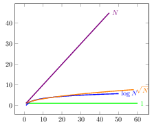
Here are run times from linear up to cubic plotted on the same graph.
Notice how close the quasilinear function to the linear.
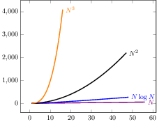
Note that $N^2$ (black) is in both graphs -- fastest growing above and slowest below.
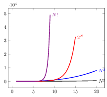
The next graph uses different scales for horizontal (1..30) and vertical axes (0..55,000).
Due to that, $N^2$ looks almost flat.
# Note on comparing algorithms on smaller inputs
As shown above, comparing algorithms depends on context and the specific parameter values.
Big‑O gives an asymptotic upper bound - how the runtime behaves as $N$ goes to infinity - so it intentionally ignores
constant factors and lower‑order terms.
For smaller inputs those ignored terms, implementation details, and hardware characteristics can change which algorithm is faster.
For example, insertion sort $O(N^2)$ frequently outperforms quicksort $O(N \log N)$ on small arrays (roughly $N \leq 50$,
but the exact crossover depends on implementation and data. When in doubt, benchmark algorithms on representative inputs.
# Using big-O to estimate run time of an algorithm
## Estimating run time of an algorithm for polynomial run times
We already used big-O to estimate run times; here are some alternative ways of doing it as well as some extra examples:
Say you have an $O(N^2)$ algorithm and you want
to know how long it will take to run on an input of size $N=100,000$. You have a week to perform the calculation.
Before you start, you want to know if it is even possible to finish the calculation within a week.
What you can do is run a small test - say $N=100$ - and measure the run time. Say it takes 1 second. Then you can estimate the run time for $N=100,000$ as follows: since run time is $O(N^2)$, it is **proportional** to $N^2$; say the actual run time is $K \cdot N^2$, where $K$ is some unknown constant.
Since we know the absolute run time for $N=100$ is 1 second, we can say:
$$
K \cdot (100)^2 = 1 \text{ second}
$$
to estimate the run time for $N=100,000$ we need to calculate
$$
\begin{align*}
K \cdot (100,000)^2 = K \cdot (100\times 1000)^2 &= \\
K \cdot (100)^2\cdot (1000)^2 &= \text{ [using the measurement from above] } = \\
1 \text{ second} \cdot (1,000)^2 &= 1,000,000 \text{ seconds} \approx 11.57 \text{ days}
\end{align*}
$$
that is one week is not enough time.
On the other hand if algorithm's run time was $O(N \sqrt N)$, then the estimation would be as follows. Initial measurement:
$$
K \cdot (100)\cdot\sqrt 100 = K \cdot (100)\cdot 10 = K \cdot (1000) = 1 \text{ second}
$$
and estimate
$$
\begin{align*}
K \cdot (100,000)\cdot\sqrt{100,000} &= \\
K \cdot 1000\cdot 100 \cdot 316.2 &= \text{ [using the measurement from above] } = \\
1 \text{ second} \cdot 31620 &= 31620 \text{ seconds} \approx 8.78 \text{ hours}
\end{align*}
$$
*Polynomial* run times are easy to work with: given a $O(n^k)$ algorithm, increasing input size by a factor of $s$ increases run time by a factor of $s^k$ (the initial input size does not matter).
## Estimating run time of an algorithm for logarithmic run times
With run times that involve logarithms and exponents the calculation is slightly more complicated.
For example given a $O(N\log N)$ algorithm that runs in 1 second on an input of size $N=2^5$, what is the run time on $N=2^6$.
Similar to above assume the actual runtime is $K\cdot N\log_2 N$. Let's calculate how much slower $N=2^6$ compared to $N=2^5$:
$$
\begin{equation*}\begin{split}
\dfrac{\text{run time }N=2^6}{\text{run time }N=2^5} =
\dfrac{k\times 2^6\log_2 2^6}{k\times 2^5\log_2 2^5} =
\dfrac{2^6\log_2 2^6}{2^5\log_2 2^5} &=
\dfrac{2\log_2 2^6}{\log_2 2^5} = \\
\text{[using the fact that } \log_2 2^k = k \text{]} &\\
2 \times \frac 65 &=
2 \times 1.2
\end{split}\end{equation*}
$$
Note the same calculation with the initial size $N=2^{20}$ and doubling to $N=2^{21}$:
$$
\begin{equation*}\begin{split}
\dfrac{\text{run time }N=2^{21}}{\text{run time }N=2^{20}} =
\dfrac{k\times 2^{21}\log_2 2^{21}}{k\times 2^{20}\log_2 2^{20}} =
\dfrac{2^{21}\log_2 2^{21}}{2^{20}\log_2 2^{20}} &= \\
\dfrac{2\log_2 2^{21}}{\log_2 2^{20}} =
2 \times \frac {21}{20} &=
2 \times 1.05
\end{split}\end{equation*}
$$
Note that factor 2 above comes from the $N$-part of $N\log N$ and does not depend on the initial $N$, while
the second is from the $\log N$-part and it does depend on the initial input size. As $N$ is growing, the second part converges to 1 - this is why $O(N\log N)$ is called *quasilinear* - it is very close to linear, and the difference becomes negligible as $N$ grows.
Same problem as above with initial $N=2^{100}$. Notice how small the second part is compared to the previous examples:
$$
\begin{equation*}\begin{split}
\dfrac{\text{run time }N=2^{101}}{\text{run time }N=2^{100}} =
\dfrac{k\times 2^{101}\log_2 2^{101}}{k\times 2^{100}\log_2 2^{100}} =
\dfrac{2^{101}\log_2 2^{101}}{2^{100}\log_2 2^{100}} &= \\
\dfrac{2\log_2 2^{101}}{\log_2 2^{100}} =
2 \times \frac {101}{100} &=
2 \times 1.01
\end{split}\end{equation*}
$$
## Estimating run time of an algorithm for exponential run times
Given a $O(2^N)$ algorithm that runs in 1 second on an input of size $N=20$, what is the run time on $N=21$?
$$
\begin{equation*}\begin{split}
\dfrac{\text{run time }N=21}{\text{run time }N=20} =
\dfrac{k\times 2^{21}}{k\times 2^{20}} =
\dfrac{2^{21}}{2^{20}} =
2
\end{split}\end{equation*}
$$
So each time we increase the input size by 1, the run time doubles. If we increase the input size by 5, the run time will
increase by a factor of 32:
$$
\begin{equation*}\begin{split}
\dfrac{\text{run time }N=25}{\text{run time }N=20} =
\dfrac{k\times 2^{25}}{k\times 2^{20}} =
\dfrac{2^{25}}{2^{20}} =
2^5 = 32
\end{split}\end{equation*}
$$
# Final remarks
- big-O notation $O(f(N))$ is a statement that an algorithm is running no slower than some constant times $f(N)$, for sufficiently large $N$. It is an **upper bound** on the run time of the algorithm. There is another notation $\Theta(f(N))$ that is a statement that an algorithm is running **exactly** as fast as some constant times $f(N)$, for sufficiently large $N$. In other words, big-O is "less-or-equal", while big-Theta is "equals". Therefore, big-O is less precise than big-Theta, but it is easier to work with (in some cases big-Theta may be plain impossible).
- when we say that our algorithm is $O(f(N))$, we mean that it (like many other algorithms) belongs to a *class* of algorithms described by $O(f(N))$.
- when stating that a function $f(N)$ belongs to a class $O(g(N))$, we write $f(N) = O(g(N))$ or $f(N) \in O(g(N))$. Even though the second notation is more precise, the first is used more often.
- if $f(N) = O(g(N))$, then $f(N)$ is also $O(h(N))$ for any function $h(N)$ such that $g(N) = O(h(N))$. For example, if $f(N) = O(N^2)$, then $f(N) = O(N^3)$, since $N^2 = O(N^3)$. We should always try to find the tightest possible upper bound, that is, the smallest class that contains our algorithm. For example, if $N^2+5N = O(N^2)$ and $N^2+5N = O(N^3)$ and so on, we should say that $N^2+5N = O(N^2)$, since $O(N^2)$ is the smallest/tightest class for $N^2+5N$.
# Flashcards - quick review
Q: What is Big‑O?
A: Big‑O is a mathematical notation that describes the upper bound of an algorithm's run time as a function of input size N. It captures the growth rate and ignores constants and lower-order terms.
Q: What are best/worst/average cases?
A: Best = minimum operations for inputs of size N; worst = maximum; average = expected over input distribution. We usually use worst-case.
Q: $O(1)$ example.
A: Constant time. Example: reading/writing a single array element `a[i]`.
Q: $O(N)$ example.
A: Linear. Example: single loop over N elements (e.g., initialization, linear search worst-case). Runtime grows proportionally to N.
Q: $O(N^2)$ example.
A: Quadratic. Example: two nested loops each up to N (matrix traversal, naive duplicate check). Total operations ≈ $N\times N$.
Q: $O(\log N)$ example.
A: Logarithmic. Example: binary search. Each step halves the search range, so iterations approximately $\log _2 N$.
Q: $O(2^N)$ example and consequence.
A: Exponential. Example: generating all outcomes of N coin flips ($2^N$ outputs). Runtime doubles when $N$ increases by 1 - becomes infeasible quickly.
Q: Rule of thumb for simplifying big-O expressions.
A: Keep the dominant term and drop constants and lower-order terms. E.g., $(N^2 + N) \to O(N^2)$; $(1/2 N^2) \to O(N^2)$.
Q: Runtime of two nested loops.
A: Multiply the counts for nested loops (assuming the count of the inner loop is independent of the outer).
E.g., two nested one up to $N$, another up to $N^2$, gives us $O(N) \times O(N^2) = O(N^3)$.
Q: Runtime of two sequential blocks.
A: Add run times. E.g., one block is $O(N)$, another up to $O(N^2)$, total is $O(N) + O(N^2) =O(N + N^2) = O(N^2)$ (since $N^2$ dominates $N$).
Q: What is an arithmetic series?
Arithmetic series - each next term is previous term **plus** constant $a_1, a_2=a_1+d, a_3=a_2+d=a_1+2d, ...$. Examples:
- 1, 2, 3, ... (here $a_1=1$, $d=1$);
- 3, 5, 7, ... (here $a_1=3$, $d=2$);
- 5, 15, 25, ... (here $a_1=5$, $d=10$).
Q: What is a geometric series?
Geometric series - each next term is previous term **times** constant $a_1, a_2=a_1 \cdot r, a_3=a_2 \cdot r=a_1 \cdot r^2, ...$. Examples:
- 1, 2, 4, 8, ... (here $a_1=1$, $r=2$);
- 3, 12, 48, 192 , ... (here $a_1=3$, $r=4$).
Q: Sum of an arithmetic series.
A: Arithmetic series sun $a_1 + \ldots a_n = \dfrac{a_1+a_n}2 \times n$. Important special case $1+2+...+N$, $a_1=1$, $a_N=N$, $n=N$, so sum = $\dfrac{1+N}2 \times N= O(N^2)$.
Q: Sum of a geometric series.
A: Geometric series sum $1+b+b^2+...+b^k = \dfrac {b^{k+1}-1}{b-1}$. Important special case
- $1+2+4+...+2^k = 2^{k+1}-1$ (since $b=2$), so sum is $O(2^{k+1})$.
- or $1+2+4+...+N$, let $k=\log_2 N$, so that $N=2^k$, then sum is $2^{k+1}-1=2^{\log_2 N +1} -1 =2N-1=O(N)$).
Q: Given two algorithms with run times correspondingly $f(N) = O(N)$ and $g(N) = O(N^2)$, which algorithm is faster?
A: **For large** $N$, $f(N)$ is a faster algorithm than $g(N)$, since $f$'s run time $N$ is below $g$'s run time $N^2$.
Q: Given two algorithms with run times correspondingly $f(N) = O(N)$ and $g(N) = O(N^2)$, which algorithm is faster for $N=10$?
A: For small $N$, it depends on the constants **hidden** in the big-O notation. Therefore big-O notations cannot provide a definitive answer for small $N$. In practice, the best way to compare is to run both algorithms on the same input (preferably multiple times on random inputs) and measure the run time.
Q: What is the runtime of the following code?
```cpp
j = i+1;
```
A: $O(1)$, since it is a single operation.
Q: What is the runtime of the following code?
```cpp
// test if N is prime by checking if it is divisible by any number between 2 and sqrt(N)
for (int i = 2; i < std::sqrt(N); ++i) { // square root
if ( N % i == 0 ) { // N is divisible by i, so it is not prime
return false;
}
}
return true;
```
A: $O(\sqrt N)$, since we are checking divisibility up to $\sqrt N$, so the number of iterations is approximately $\sqrt N$.
Q: What is the runtime of the following code?
```cpp
for (int i = 0; i < N; ++i) {
cout << a[i] << " ";
}
```
A: $O(N)$, since we have a single loop that iterates N times.
Q: What is the runtime of the following code?
```cpp
for (int i = 0; i < N; ++i) {
for (int j = 0; j < N; ++j) {
cout << a[i][j] << " ";
}
}
```
A: $O(N^2)$, since we have two nested loops, each iterating N times, so total iterations are $N \times N = N^2$.
Q: What is the runtime of the following code?
```cpp
while (N > 0) {
cout << N << " ";
N /= 2;
}
```
A: $O(\log N)$, since we are halving N in each iteration, so the number of iterations is approximately $\log_2 N$.
Q: What is the runtime of the following code?
```cpp
while (N > 0) {
cout << N << " ";
N /= 2;
}
```
A: $O(\log N)$, since we are halving N in each iteration, so the number of iterations is approximately $\log_2 N$.
Q: How much longer will input size 20 take compared to 10 for a $O(1)$ algorithm?
A: Same time, since $O(1)$ means constant time regardless of input size.
Q: How much longer will input size 30 take compared to 10 for a $O(N)$ algorithm?
A: Approximately 3 times longer, since runtime is proportional to N (30/10 = 3).
Q: How much longer will input size 50 take compared to 10 for a $O(N^2)$ algorithm?
A: Approximately 25 times longer, since runtime is proportional to $N^2$ ($(50/10)^2 = 25$).
Q: How much longer will input size 30 take compared to 20 for a $O(2^N)$ algorithm?
A: Approximately 1024 times longer, since runtime **doubles with each increase in N by 1** so it will double 30-20=10 times, for a total of $2\times 2 \ldots \times 2 \text{(10 times)} = 1024$.